This month we continue our look at Graphical Function Diagrams (GFD). GFD’s help us visually see how two variables are interrelated by plotting the relationship between the two over the range of relevant values.

In Chaos: Making a New Science (Penguin Books, New York), James Gleick describes a relatively new branch of science that has profound implications for how we view our world. Chaos, simply put, is the science of seeing order and pattern where formerly only the random, erratic, and unpredictable had been observed. In a way, systems thinking also deals in the science of chaos. Diagrams such as causal loops, accumulators and flows, and graphical functions arc all ways of extracting the underlying structure from the “noise” of everyday life.

Relating Behavior to Structure

Both systems thinking and chaos insist that real-world phenomena need to be described in “real” terms that match our intuition. Writing partial differential equations to describe clouds, for example, misses the point, because we don’t perceive clouds in that way. It is not enough to have a model that reproduces some real-world phenomena if we cannot identify the structures that produce the behavior of the actual system. That’s why systems thinking diagrams focus on capturing reality in a format that taps into our intuitive understanding of the systems which we manage and live in.

Savings Loop

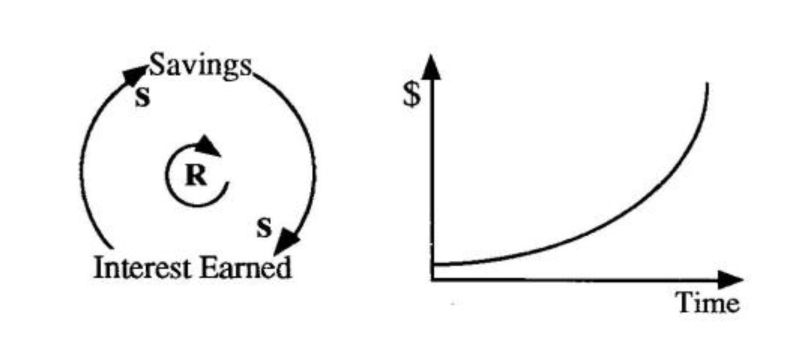
If we begin to explore our savings account “system” by drawing a causal loop diagram, we see that an increase in savings will lead to more interest earned, which increases our savings balance still further (left). The graph of this behavior over time will look something like the exponential growth curve (right).

From Causal Loops to GFD’s

To see how a range of systems thinking tools can help capture the structure of a system at increasing levels of detail, let’s look once again at a system we are all familiar with — a savings account. If we plot out the structure of a savings account using a causal loop diagram (see “Savings Loop”), we see that an increase in savings will lead to more interest earned, which increases our savings balance still further. The graph of this behavior over time would look something like the exponential growth curve shown on the right of the diagram.

“Wait a minute,” you may protest, “I don’t know whose bank account that is, but it certainly doesn’t look like mine!” That’s true — rarely is a system so simple in real life; nor are bank accounts that well-behaved. There are usually many other factors involved. The question of how many factors to include always depends on the purpose of examining the system. Since the details of any system are infinitely complex, it is futile to strive to “model the system.” In our sample case, the purpose is to represent as concisely as possible the important factors which affect the balance of a typical savings account, so we want to look at savings, income, interest earned, and spending (see “Savings & Spending Loops”). If we were only interested in capturing the fact that there is a balancing loop that explains the slowdown in the growth of our savings account, we could stop at this point. On the other hand, if we want to be more explicit about the structure behind the behavior, we need to translate our diagram into accumulators and flows.

Savings & Spending Loops

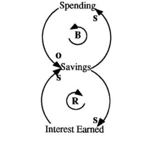
A balancing loop explains the slowing growth of the savings account: as our savings increases, we are more likely to increase spending, which will reduce our savings.

Accumulators and Flows

When we translate CLD’s into Accumulators and Flows, we are becoming even more precise about the structures producing the dynamics. The bathtub as a metaphor for accumulations (see “Accumulators: Bathtubs, Bathtubs Everywhere,” Toolbox, February 1991) helps us visualize how concepts as diverse as savings, pollution, customers, and corporate reputation share a similar underlying structure.

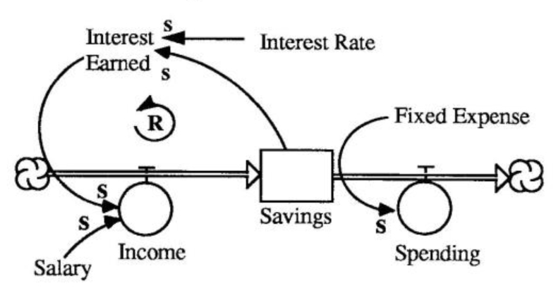
Accumulators and flows add more detail and understanding to our causal loop diagram by differentiating between those variables in the diagram that “accumulate” (our savings balance) and those that just “flow” through the system (income and spending). In the “Savings as an Accumulator” diagram, we can visually see money flowing into and out of savings in the form of income and spending. More importantly, we can relate to this structure intuitively because we experience money in terms of flows and accumulations (or lack thereof!).

Graphical Functions: Mapping Policies

So now we have a pretty good idea of both the basic dynamic behavior of the savings account, and a feel for the important inflows and outflows. But our model is still pretty elementary. Suppose now you wanted to go a little further and use a systems diagram for describing your family’s policy for managing your savings. “Our discretionary spending depends on how much savings we have,” you explain. “If the balance in our savings account is below $5000, we don’t spend a dime. As our savings rise above $5000, we may increase discretionary spending by, say, $15-20 per month. If our savings tops $10,000, then we’re likely to spend several hundred dollars a month. But in any case, we don’t see ourselves spending more than $500 per month on discretionary expenses.”

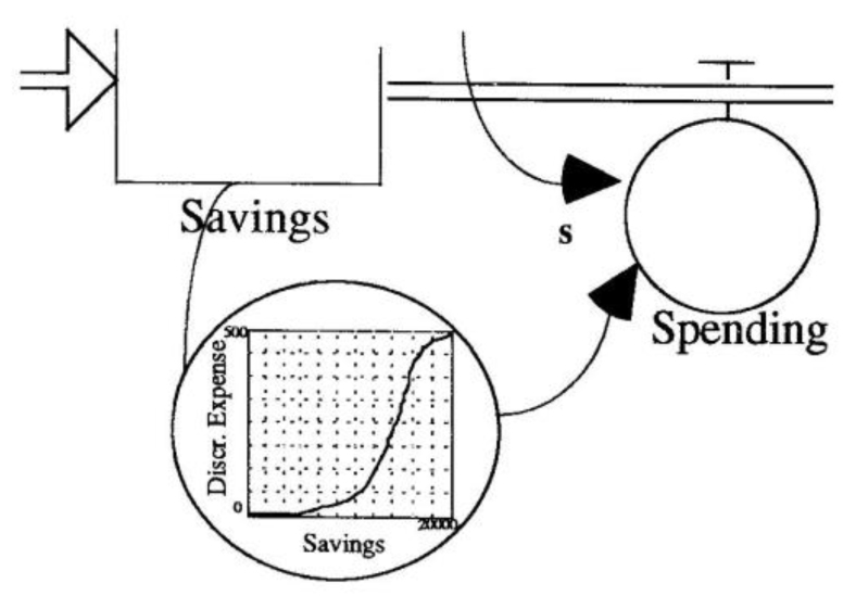
Graphical functions allow us to expand our exploration of a system to include policies and interrelationships between variables. If we tried to capture the savings plan we described above in an analytical form we would have to do quite a bit of work in order to come up with a suitable equation. And when we were done, it would be hard to tell if the equation represented our savings account or the number of widgets on sale at Wal-Mart. The truth is, most of us don’t think in terms of abstract mathematical concepts, but in images and structures grounded in our everyday experience. That’s why graphical functions are useful. They capture policies in an intuitive way through a simple graph that maps out the relationship between one variable in relation to another (see “Savings Policy Graphical Function Diagram”). In our savings policy plan, for example, we see at a glance that savings has no impact on our discretionary expenses until savings hits $5,000. After that, discretionary expenses rise until savings reaches $20,000, at which point they level out at $500.

Artistic Managers

Physicist Mitchell Feigenbaum suggests that art is a theory about the way the world looks to human beings. “It’s abundantly obvious that one doesn’t know the world around us in detail. What artists have accomplished is realizing that there’s only a small amount of stuff that’s important, and seeing what it is.” Whether we recognize it or not, we are artists as well, selectively picking out details of the world which we choose to focus on. Those details appear as items on our production reports, financial statements, and customer surveys. To the extent that those details do not capture the core structures that are important, we may be the unwitting producers of our own chaos. As one systems thinking maxim warns, “It ain’t what you don’t know that hurts you, it’s what you DO know that ain’t so.”