Last month we outlined a process for turning a causal loop diagram into an accumulator and flow diagram, using the example of staffing decisions. Now we want to bring that diagram to life through a computer simulation model and see how the identified relationships interact over time.

1. Specify Numeric Values

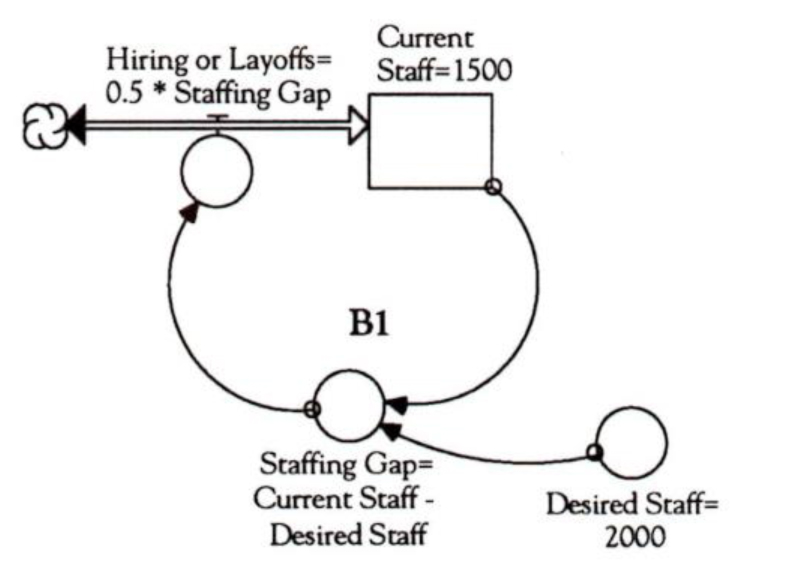
The first step in bringing our diagram to life is to assign quantities to the policies and decisions that are mapped in the diagram. For example, let’s say our current staff is 1500 people and our desired staff is 2000. A question we need to consider is, “How quickly do we want to close the gap?” The aggressiveness of our time horizon will determine the flow of people in and out of “Current Staff.” Let us assume that we want to close one-half of the gap each month. We could then define “Hiring or Layoffs” as 0.5*Staffing Gap (see “Defining the Variables”).

2. Check for Consistent

After assigning numerical values, we should conduct a quick check to make sure we have defined the variables correctly and that the dimensions are consistent. For example, both our current staff and desired staff will be measured in numbers of people, as will the staffing gap (the number of people needed to close the gap). The “Hiring or Layoffs” flow should represent the number of people flowing into or out of the company over a period of time (people/ month). From our quick check, it looks like the variables are all consistent (people and time). If we had found one variable with a different measurement, such as dollars, it would signal a need to recheck our definitions.

3. Check for Delays

Since delays play an important role in the dynamics of any system, we need to make sure they are captured explicitly in the computer model. Our original story mentioned several significant delays: the time it takes to recognize the gap between current and desired staff, the delay before deciding to act on it, and the time it takes to actually hire or lay off staff. Suppose we know that it takes approximately three months to hire and train a new person. We can include this information in the computer model either by using a built-in delay feature found in most software packages, or by modeling it explicitly with an additional stock.

4. Determine Time Horizon of the Simulation

One of the lessons learned from years of computer simulation work is that we often underestimate the time necessary for the dynamics of a system to play out. A good rule of thumb is to let the simulation run three to five times as long as the longest explicit delay in the system. Since we know there is a three-month delay between the recognition of a staffing gap and when people actually come on board, we want our simulation to run at least nine to 15 months. To appreciate more fully the long-term dynamics, we will let it run for two years.

5. Build Confidence in the Model

Before actually experimenting with different policies in the simulation, we want to build our confidence that the model is an accurate representation of the system we are studying. One way to determine if the model is robust is to conduct a series of simple tests to verify that simulation results match real or historical data of what we know or expect will happen. If, for example, our current staff is 2000 people and our desired staff is also 2000 people, we would expect that no hiring or layoffs would occur. Running that test should produce a straight line. If, however, the graph of “Current Staff” bounces around or increases, the model needs to be checked for errors.

6. “What If” Scenarios

Asking whether something will happen can lead to non-productive conversations about why one outcome is more likely than another. But when we ask what if something were to happen, we can enter into a productive exploration of the possible consequences.

Defining the Variables

The first step in bringing our accumulator and flow diagram “to life” is to define the policies and decisions that are mopped in the diagram so we can see how they will play out over time.

Therefore, once we have confidence in the model, we want to run a “base case” scenario to see if we get any interesting insights into the structure. For example, if we try to close one-half of the gap each month with a three-month delay for each new hire, we discover that we overshoot and oscillate around our target number of 2000 (see “‘What If’ Scenarios”). We end up hiring more people than we need because our hiring policy and the number of “Current Staff” doesn’t account for people we have already begun to hire.

We may also ask what would happen if we shortened the delay in the hiring process itself, instead of trying to increase the number of people we hire. Let’s say we make a real push to get people on board in two months (by resetting our delay function to two months instead of three). What would we expect? As the graph shows, this goal would allow us to approach our target employee number more smoothly.

Another scenario we can explore is changing our level of aggressiveness — let’s say we will try closing 100% of the gap each month (“Hiring and Layoffs” = l*Staffing Gap). What do we expect to happen? The result may be surprising — we will overshoot the target by a much greater number. This scenario creates larger oscillations because the number of people-in-process that are unaccounted for is greater.

What If Scenarios

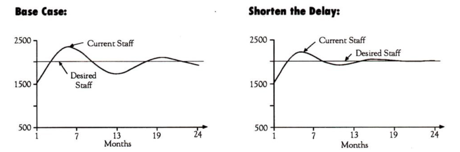
These two scenarios compare possible staffing strategies. As the right-hand graph shows, shortening the hiring delay to two months allows us to approach ow target number more smoothly.

Consider the Pipeline

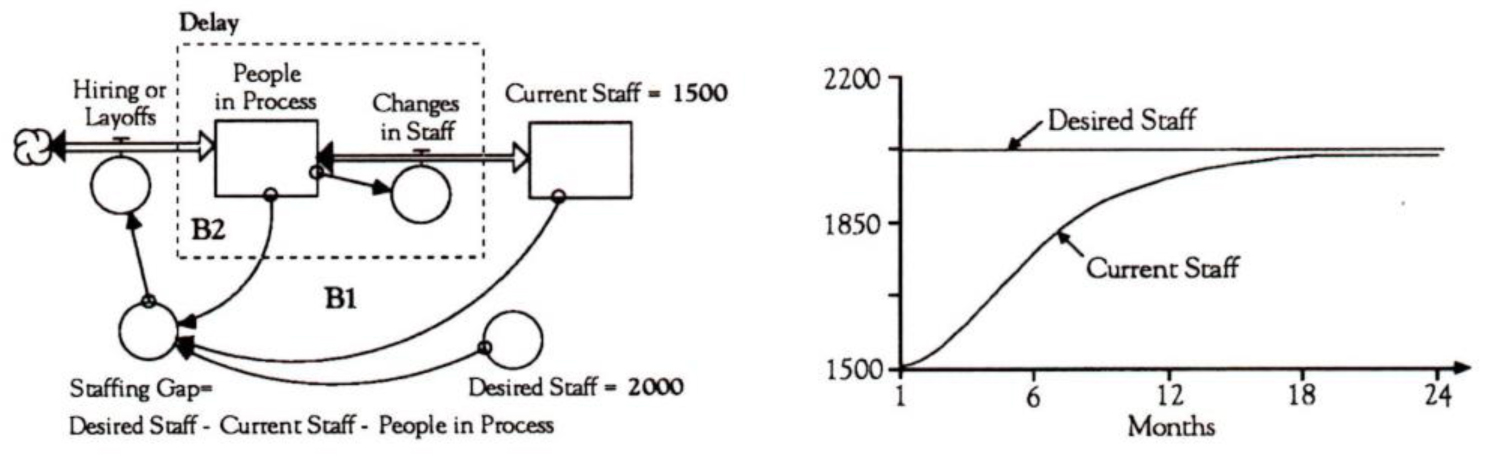
If we account for the pipeline of “hires in progress” when we compute the staffing gap, we actually alter the structure by adding a new balancing process (82). This will allow us to close the staffing gap smoothly.

Is there a way to eliminate the oscillations altogether? What if we account for the number of people already in the hiring pipeline when we compute the gap? By changing our model to make the delay more explicit — as a pipeline of people in process — we can test this scenario (see “Consider the Pipeline”). If we run this simulation with the assumption that we will close one-half of the gap each month (“Hiring or Layoffs”= 0.5*Staffing Gap), we will in fact eliminate the oscillations. By accounting for the pipeline, we are actually altering the structure by adding a new balancing loop (B2).

Learning Curve

Although our staffing issue is a somewhat simplistic example, working through these steps forces us to articulate and test our beliefs about a problem, offering a way for us to refine our mental models. For this reason, modeling is a very powerful tool. However, the learning curve for modeling can be steep. You can teach someone to use a modeling program in a few hours, but learning how to design a model that produces usable results and advances a team’s learning requires a much more significant investment. Constructing good computer models, like drawing good causal loop diagrams, requires the inclusion of multiple perspectives, the commitment to surface and challenge our mental models, and continual practice.

This article is based in part on “Moving Into Computer Modeling” by Michael Goodman, which appeared in The Fifth Discipline Fieldbook (Doubleday, 1994). For more information about the various modeling programs available, see pages 547-548 of The Fifth Discipline Fieldbook.

Michael Goodman is vice president of Innovation Associates (Framingham. MA) and a frequent contributor to The Systems Thinker. He has been involved in the field as oxi educator and consultant for over 20 tears.

Editorial moon for this article was provided by Colleen Lannon-Kim.