TEAM TIP
Look for things that rise and fall in your organization, such as employee motivation, product sales, progress on goals, etc. What are the balancing loops that control and limit growth in these areas?
In part one of this series, I stated, “A mental model is a model that is constructed and simulated within a conscious mind.” A key part of this definition is that mental models are not static; they can be played forward or backward in your mind like a video player playing a movie. But even better than a video player, a mental model can be simulated to various outcomes, many times over, by changing the assumptions.
Mental Simulation
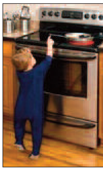
Remember the example from part one of the child reaching for the hot stove? One possible outcome we can simulate is that the child does not get burned. We can simulate this outcome by altering our assumptions. We could include a parent in the room who rescues the child in the nick of time. Or, we could simulate the child slipping just before reaching the stove-top because, in the photo, the hardwood floor appears slippery. This kind of mental simulation allows us to evaluate what may happen, given different conditions, and inform our decision making. You don’t have to make any decisions while looking at the picture, but imagine what actions you might take if the scene above was actually unfolding in front of you.
It seems effortless to mentally simulate these types of mental models. Most of the time, we are not even aware that we are doing it. But other times, it becomes obvious that our brain is working rather hard. For example, looking at the chess board below, can you determine if the configuration is a checkmate?
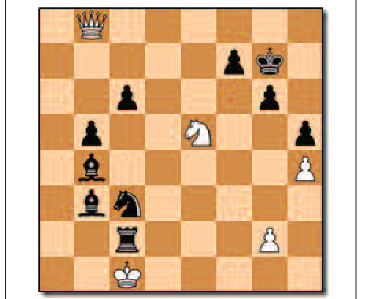
It is indeed. But I’ll bet it took noticeably more effort for you to mentally simulate the chess game than it did with the child near the stove scenario. Think about the mental effort that the players make trying to simulate the positions on the board just a few moves ahead in the game.
The paper “The Magical Number Seven, Plus or Minus Two: Some Limits on Our Capacity for Processing Information” by G. A. Miller (1956) established that people can generally hold seven objects (numbers, letters, words, etc.) simultaneously within their working memory. Think of “working memory” as you would think of memory in a computer. It’s like the amount of RAM we have available to perform computations within our mind. And it’s not very much. This means if people want to do any really complex information processing, they’ll need some help. Over the last 50 years or so, the help has come from computers. (In fact, IBM designed a computer specifically for playing chess, dubbed “Deep Blue”).
Digital computers have catapulted humankind’s ability to design, test, and build new technology to unbelievable levels in a relatively short period of time. Space exploration, global telecommunication, and modern healthcare technology would not have been possible without the aid of computers. We are able to perform the computation required to simulate complex systems using a computer instead of our minds. Running simulations with a computer is faster and more reliable.
What Makes a Model Useful?
Models that we can simulate using computers come in many forms. For example, a model could be a financial model in a spreadsheet, an engineering design rendered with a CAD program, or a population dynamics model created with STELLA. But what makes any of these models useful? Is it the model’s results? Its predictions? I think the ability to explain the results is what makes a model truly useful.
Models are tools that can contribute to our understanding and decision-making processes. To make decisions, a person needs to have some understanding of the system the model represents. A business finance model, for example, can be a useful tool if you understand how the business works.
Consider a model that does not provide any explanatory content, only results. This type of model is often referred to as a “black box.” It gives you all the answers, but you have no idea how it works. People rarely trust these types of models, and they are often not very useful for generating understanding.
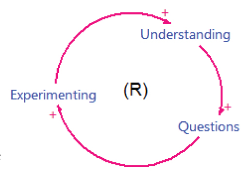
The most useful models are structured so that the model itself will provide an explanatory framework that enables someone to ask useful questions of it. Those questions may be answered by experimenting with the model (simulating) which, in turn, can help deepen a person’s understanding of the system.
This is an important feedback loop in a person’s learning process. This feedback loop can be accelerated if the model provides explanations and can be simulated with a computer.
Transforming your mental models into visual models that are easier to understand and experiment with will deepen your understanding and help you communicate your models more effectively.
Modeling Dynamic Systems
Dynamic systems are notoriously difficult to understand. A survey of opinions and policy proposals concerning the recent global economic crisis, healthcare reform in the US, and climate change will yield a myriad of mental models about how these systems work, and what action we can take to improve them. These systems are hard to understand because they challenge our mental capacity to model and to simulate them. Systems problems are characterized by non-linearity, delays, and competing feedback loops, all of which are challenging to understand.
As a result of the complexity that is inherent within dynamic systems, you’ll often find a lot of debate and mistrust of proposals to change them. Think about how complex issues are presented in newspapers, in blogs, on television, and in the workplace. Typically, projections concerning what will happen if we adopt one proposal or another will be presented with little explanation of how the proposal will change the system’s behavior. People have difficulty engaging in meaningful discussion about how to actually solve problems without any common ground for understanding the dynamics of the system.
This is why developing a visual representation of how a system is structured underpins the philosophy behind systems thinking and simulation software such as iThink and STELLA. In this article, I’ll show how this works using STELLA.
Stocks and Flows
The mental model of the learning process pictured above is a visual representation of cause and effect relationships. These cause and effect relationships can be modeled operationally using stocks and flows to simulate them using STELLA.
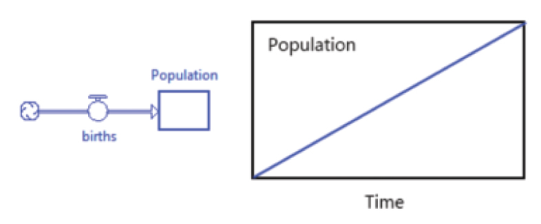
A stock is an accumulation within a system. Think of it as a bathtub. Like a bathtub, stocks can be filled and drained. In STELLA, stocks are indicated by a rectangle. Stocks can be anything that accumulates— water, money, people, anger, and motivation are all examples of stocks.

A flow can add to, or subtract from, a stock. Think of the faucet running water into the bathtub as it fills. The stock is the accumulation of water in the bathtub, and the flow is the rate at which the water is flowing in.
In the example below, the Population stock increases as people are born. If people are born at a constant rate, then we’ll see a linear increase in the Population over time.
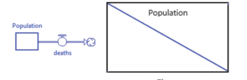
Similarly, the deaths flow pictured below removes people from the population, causing the level to drop over time.
The clouds on the ends of the flows represent infinite sources or sinks. In the model above, deaths flow into a cloud, which is outside the system boundary and therefore can accumulate infinitely.
Feedback Loops
Feedback loops are what enable systems to run themselves. They are difficult to simulate mentally, but easy to construct using stocks and flows. A connector (red arrow) indicates a dependency between two parts of a system. In the model below, the births flow is dependent on the Population level and birth rate.
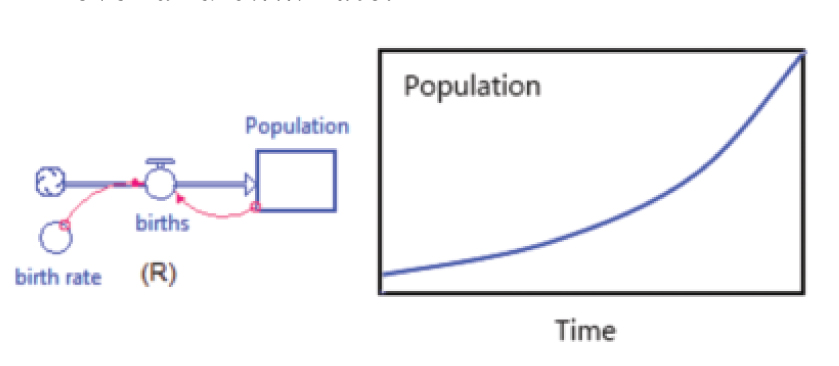
The birth rate is represented using a converter. Converters can contain expressions or constants that can be used to modify other parts of the model. As you might suspect, the births flow is defined as Population * birth rate. By representing the birth rate with a converter, we can easily see that the flow of births is a function of both Population and birth rate.
This structure creates a reinforcing feedback loop. Notice the population exhibits exponential growth when simulated over time. There is nothing limiting the growth of the population. One way to limit the growth is to add a balancing loop.
The relationship between the size of the Population and the death rate form a balancing loop. The death rate changes based on the Population size and therefore limits the growth of the population. If the population grows too dense, deaths occur at a higher rate.
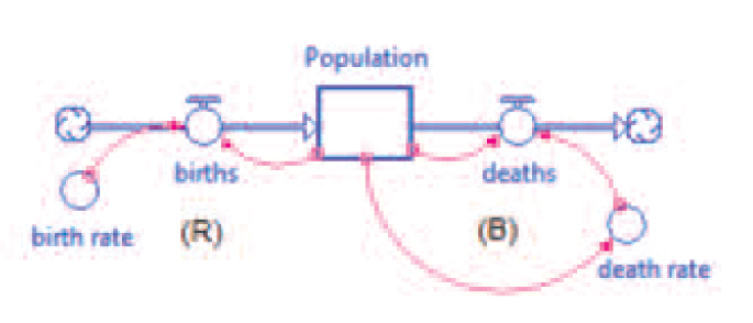
Now that we have explored the basic building blocks (stock, flow, connector, converter) and how to map out feedback loops, we can build, and experiment with, a real model of a complex feedback system.
Predator-Prey Dynamics
A classic example of a complex feedback system is the dynamics exhibited by predator-prey populations. A remarkable dataset from the Hudson Bay Company in Canada of lynx and snowshoe hare pelt trading records gives us a rare look at an isolated natural system. The records span almost a century, beginning in 1845. From these records, we can infer the population levels of both species.
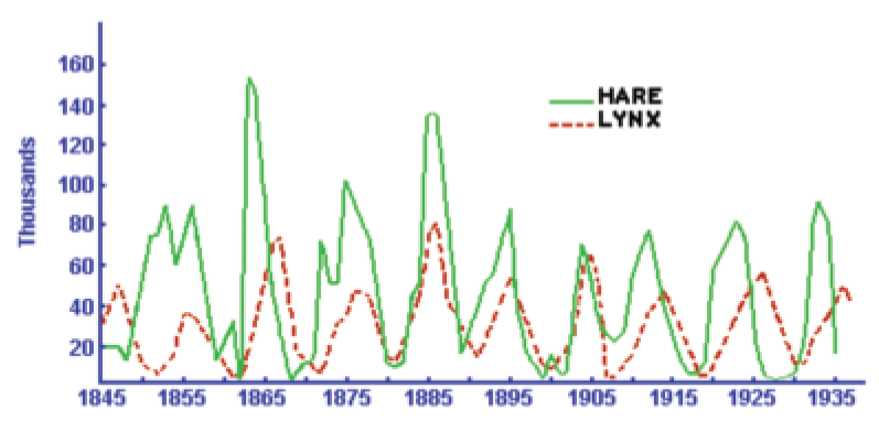
At first pass, it seems that there was little keeping the hare population in check other than the lynx population (hares are the primary food source for lynx). What is interesting here is the oscillation pattern. How does the interaction between the two population systems generate this oscillation? Let’s try to answer this question by constructing a model that we can easily understand and experiment with.
Understanding the System
What is your mental model of how a lynx population increases or declines over time? My guess is that it may include a long list of external factors (industrialization, weather, urban sprawl, etc.), but the core of the mental model probably contains operational understanding: Births and deaths ultimately control the population level. Converting this mental model into an operational stock and flow model in STELLA looks like this:
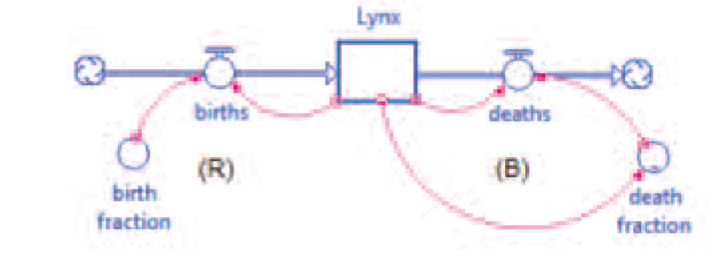
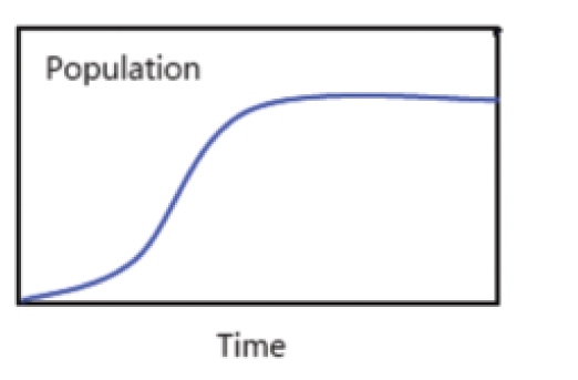
The more lynx you have in a given population, the more lynx are born. This is a reinforcing feedback loop. As the population increases, lynx may start dying at a faster rate because they run out of some resource, such as food. This is a balancing feedback loop. Here are the results after I run the simulation:
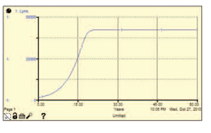
We can see the population exhibits S-shaped growth. The value at which the population levels off is the number of lynx that is sustainable within this particular system.
This simple model is congruent with most people’s mental models of population dynamics: The population grows or declines based on the limits of what is required to sustain it. But let’s go a bit deeper and think about how this works. What we have modeled is two feedback loops (reinforcing and balancing) competing with one another.
The graph above illustrates that the reinforcing feedback loop dominates at the beginning of the simulation, but as the population grows, the balancing loop takes control and dampens the growth. Lynx are still being born when the population level stabilizes; it’s just that the number of deaths has become equal to the number of births. Sometimes a balancing loop is referred to as a “goal-seeking loop.” The level of the stock stabilizes when the goal is met.
Take a moment to think about how the feedback loops within the lynx and hare populations could interact with one another to generate the oscillation we saw. We know that each population in isolation will grow until the carrying capacity of the system limits it. What would happen if we modified the model diagram to show the dependency between the lynx and hare population?
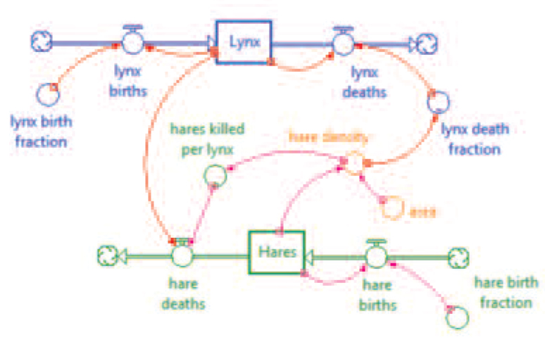
I have connected the Lynx population with hare deaths and the stock of Hares with lynx death fraction via the hare density variable. (The lynx death fraction changes based on the density of hares in the given area.) I now have a useful model of a complex system: It is easy to understand how the model is structured, and I can experiment with the model by simulating different scenarios.
Experimenting
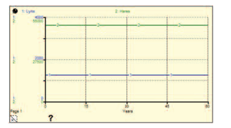
I have initialized the values in the model so that it begins in “dynamic equilibrium”— lynx and hares are dying and being born, but the population levels stay the same. This is like a bathtub that has the faucet running at the same rate as the water leaving through the drain. The level stays constant, but water is cycling through. In this case, we have many generations of lynx and hares, but within the respective populations, the number of births and deaths are equal.
If we begin with the model in a steady-state, we’ll easily recognize change in behavior as we experiment. Let’s explore the impact of trapping on the populations, since we know both species were trapped for pelts when the data was collected.

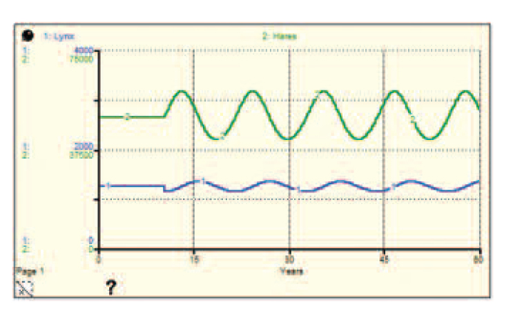
I have added an additional outflow to the stock of Lynx that represents trapping. I defined the outflow so that trapping begins after 10 years. At that point, 100 lynx are trapped and removed from the stock of Lynx. Pictured below is the graph after the simulation is run with this new scenario:
And here is the graph after I set lynx trapped to 500 and ran the simulation again:
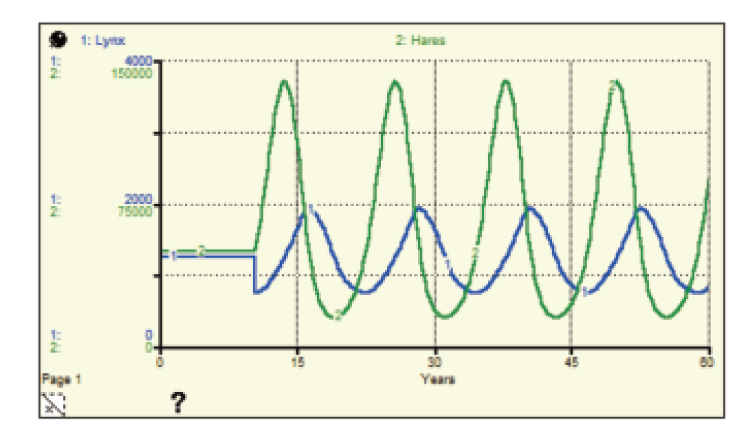
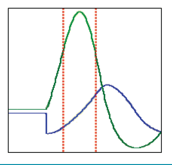
In both experiments, the populations begin oscillating at the moment the trapping suddenly reduces the lynx population. How can our knowledge of the feedback loops at play in this system help explain these results? We know that in this model, the size of the hare population is limited only by the number of lynx. When that number suddenly drops, the hare population increases because there are not as many lynx hunting the hares. What happens to the lynx population? Because there are more hares and fewer lynx, the lynx population increases as well. (There is ample food available for the reduced lynx population.) The reinforcing loop of births increases the population level, unconstrained by its balancing loop (Figure 1).
FIGURE 1
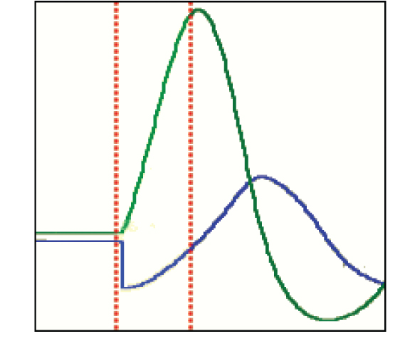
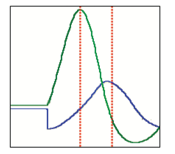
Then something interesting happens: The hare population peaks as the lynx population reaches its pre-trapping level. At this point, the lynx population has increased to a level that limits the growth of the hare population (Figure 2). Lynx are eating hares faster than they can reproduce because of the increased hare density and number of lynx hunting. In other words, the hare population’s balancing loop is limiting hare growth.
FIGURE 2
For a few years following the hare population’s peak, the lynx population continues to grow. During this period (as the hare population falls and lynx population rises), the reinforcing births loop dominates the lynx population level (Figure 3). There are ample hares available to prevent the lynx population from starving; the lynx balancing loop is not limiting their growth.
FIGURE 3
A few years later, the lynx population’s balancing loop kicks in as the number of hares plunges downward. There are not enough hares left to support so many lynx, so they die at a much faster rate. This rapid decline in lynx has the same effect on the hare population as trapping lynx: It begins another cycle of the populations overshooting the carrying capacity of the system, and subsequently collapsing.
How did our understanding of the model structure help us understand the results of our experiments? We traced the cause of the oscillation back to the behavior of the feedback loops at play within the population systems. In doing so, we gained a deeper understanding of the system that includes the behavior of two interdependent balancing loops. This understanding can lead to more questions: Will we observe the same behavior if we trap hares instead of lynx? How can we stop the oscillation? How will the oscillation change if we include the hare population’s food constraint in the model?
In the early 1900s, the mathematicians Lotka and Volterra came up with a pair of non-linear, differential equations to describe the dynamics of a predator-prey system. (They did not have the luxury of computers and software). The same oscillating behavior is observed in economic systems, and as a result the Lotka-Volterra equations played a role in the development of economic theory. It is the understanding of the dynamics of oscillation that is useful here — much more so than the numbers. This understanding enables us identify the structures that cause this behavior. When we observe oscillatory behavior in the future, our mental models will be more accurate, and we’ll be better equipped to make an informed analysis.
Better Mental Models, Simulated More Reliably
Our world is only going to become more complex, and we need good thinkers helping to make it a better place for everyone. Sharing systems models with people is a great way to increase their understanding of feedback loops and system dynamics. Building models yourself is even more valuable, because you’ll learn a lot about your own mental models and improve them. Practice will help you to construct better mental models, simulate them more reliably, and communicate them more effectively. Improving these skills will help inform what actions you take in the face of complex, systemic problems.
Jeremy Merritt is a lead software engineer at i see systems, Inc. This article originally appeared on the Making Connections blog and is reprinted with permission.