Perhaps you’ve read about system dynamics but not been ready to invest in a commercial simulator to test your ideas. Perhaps you use a commercial simulator such as ithink®, Stella®, Vensim®, or Powersim® but find it limiting in certain situations. There are alternatives. You’ll need to have — or to work with someone who has — a bit of experience programming computers using the C language. If you fulfill that prerequisite, you can start easily, and you’ll gain familiarity with tools that have broad applicability.
We’ll use paper and pencil (the only items you’ll have to pay for, assuming you own a fairly up-to-date computer) to sketch out the initial model, a simulator called SimPack to code the model, a compiler called gcc to compile the model into an executable program, gnuplot for the graphics, and Dia for producing stock and flow diagrams and other documentation (see “Shoestring Resources”).
The Process, Briefly
Let’s start with model building. I still find paper and pencil the best way to get started — it’s easy to use, there is no syntax checking to constrain creativity, and editing is quick and satisfying — erase small mistakes or, for bigger changes, ball up the paper and throw it in the recycling bin.
Once you have sketched a model, it’s time to convert it into something the computer can understand. While it’s not too hard to write a basic system dynamics simulator from scratch, SimPack, a collection of simulation programs produced by Paul Fishwick at the University of Florida, makes life easier.
SimPack provides two system dynamics simulator programs that you’ll find in the constraint/differential/integrate subdirectory of SimPack: conte.c for Euler integration and contrk.c for Runge-Kutta integration. You’ll need to enter your model equations as statements in the C programming language.
Once you’ve coded the model in C, you’ll need to compile it to turn the C program into an executable program for your computer. If you’re running on Linux or Mac OS X, you probably have ready access to the compiler gcc. If you’re running Windows, Cygwin offers a free environment that includes gcc and other tools you might use.
After you compile and run the program, you’ll get a file full of numbers, representing the value of each variable of interest at each point of simulated time. Gnuplot can graph that data.
What’s left? Perhaps you want to communicate your thinking about the relationship between stocks and flows in the system to others. Use Dia to create traditional or creative stock and flow diagrams. Both Dia and gnuplot can produce results suitable for casual viewing on the screen, incorporation into a Web site, or publication in a report or journal.
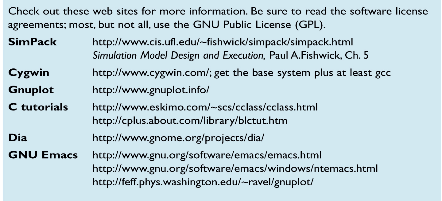
SHOESTRING RESOURCES
Taking the Next Step
If you haven’t programmed much, you may be a bit overwhelmed. Move forward in small steps. Start by installing and exploring gnuplot and Dia; you’ll likely find many uses for them, including plotting data and drawing diagrams.
Then install Cygwin, if you’re on Windows. While it can be a massive download, all you really need is the basic installation plus gcc. You’ll probably want the man (manual) pages, too.
Even if you decide you prefer to use a commercial simulator, you might find that some of these tools can augment your normal processes. For example, I’ve used gnuplot to produce publication-quality graphics from data generated using a commercial simulator.
Who knows? You might enjoy systems thinking on a shoestring!
Bill Harris (bill_harris@facilitatedsystems.com) is principal and founder of Facilitated Systems, a company dedicated to helping organizations address complex problems, work more productively in meetings and groups, and learn more effectively from experience.
this is a continuation…
Making It Concrete
The Model. To illustrate, I’ll carry a simple model about the spread of infection through a population through the entire process. If you need more information, refer to “Shoestring Resources” in the main article.
The SI model is a simple model of disease. It divides a population into two groups: Susceptible (S) and Infected (I) people (thus the SI moniker). There’s only one flow, from S to I. The number of susceptibles becoming infected per day, ipd, is the product of the number of susceptible people S, the number of contacts a susceptible person has per day c, the probability of any one contact being with an infectious person, and the probability of getting infected from contact with an infected person p:
ipd = S * c * (I / (S + I)) * p
For more information, see chapter 9 of John Sterman’s Business Dynamics (McGraw-Hill/Irwin, 2000).
To create the simulation program, open the SimPack file conte.c in a text editor (e.g., Notepad; I use GNU Emacs) and save it as si.c in a convenient directory. Then set the number of initial susceptibles S to 9999, the number of initial infecteds I to 1, the probability of getting infected from one contact p to 10% (0.1), and the number of contacts per day c to 4 by editing the initialization function init_conditions in si.c:
init_conditions() { out[1] = 9999.0; /* Susceptibles */ out[2] = 1.0; /* Infecteds */ p = 0.1; c = 4.0 time = 0.0; delta_time = 0.125; } Note that we don’t refer to S and I by those names; rather, we use elements of the array in and out to represent values of stocks. out[1] holds S, the number of susceptible people just calculated by the model, while in[1] holds the value of S to be used at the start of the next iteration. The function init_conditions also sets the initial time to 0 and the simulation time increment (often referred to as DT in system dynamics models) to 0.125.
We need one more SimPack function to calculate the results:
state() { /* Calculate flows */ ipd = out[1] * c * (out[2] / (out[1] + out[2])) * p; /* Update stocks */ /* Susceptibles */ in[1] = 0.0 – ipd; /* Infecteds */ in[2] = ipd – 0.0; }
We have a bit of housekeeping to attend to, as well; we’ll need this declaration at the start of the program:
double d, c, ipd;
In the function main, we’ll set the program to run when time (in days) is less than 50.0, and we’ll add a statement to print out all the results. To speed experimentation, I print all the stocks and flows and let gnuplot select the values to plot:
printf( “%f %f %f %f n”,time, out[1], out[2], ipd);
If you’re not a C programmer, some of this may look like gobbledygook; you can just try it, or you can read some of the “Shoestring Resources.”
Compile this program by typing two simple commands in a Cygwin command shell window:
gcc –o si.exe si.c ./si.exe > si.dat
The first line compiles the program si.c, creating si.exe, and the second runs si.exe, putting its results in the file si.dat. Si.dat has four columns: the time, S, I, and ipd. You can look at si.dat with your favorite text editor to see the results. If you’ve made it this far, pat yourself on the back; you’ve created a system dynamics model!
Plotting the Output
Few of us are satisfied looking at such a long list of numbers. Start gnuplot, and enter the command
cd “/Documents and Settings/My Documents/My Name/”
if that’s where you put your program. Then the command
plot “si.dat” using 1:2
will plot the number of susceptible people over time.
plot “si.dat” using 1:3
will plot the number of infectious people over time.
plot “si.dat” using 2:4
will create a phase plot showing the number of people getting sick per day for different values of the susceptible population. In each case, the numbers in the plot statement refer to columns in the data file you wrote when you ran si.exe.
Gnuplot can plot multiple graphs on the same sheet and can format the output for the screen or publication.
Making Life Simpler and More Powerful
As you advance, you’ll likely need a table function to represent nonlinearities. With basic C programming skills, it isn’t hard to create. You might also want to be able to give your model new parameter values without recompiling the program; the getopt C library function can help. If you want to reduce the typing required for this work, check out gnuplot mode for the Emacs text editor in the “Shoestring Resources” section of the main article.
Stock and Flow Diagrams. Those of us accustomed to using commercial simulators expect to see computer-generated stock and flow diagrams. We’ll use Dia. While you can draw straightforward stock and flow diagrams easily with Dia, you can also exercise a bit of creativity, using a symbol for stocks that suggests the type of object being accumulated and a symbol for flows that matches the symbol for stocks.
Now that you’ve seen that you can do system dynamics on a shoestring, remember all the good practices you’ve learned elsewhere. Happy modeling!
Bill Harris (bill_harris@facilitatedsystems.com) is principal and founder of Facilitated Systems, a company dedicated to helping organizations address complex problems, work more productively in meetings and groups, and learn more effectively from experience.